Mastering Excel’s XLOOKUP() function

The introduction of the XLOOKUP() renders the VLOOKUP() & HLOOKUP() functions redundant. Don’t celebrate yet: the XLOOKUP() function is most definitely not as easy to use as its predecessors! This tutorial is based on the VLOOKUP() tutorial so that we can easily compare the two.

1. Syntax

The syntax is fairly complex, so for now, I recommend skipping over this part and going straight to the Example below — the initial example skips all but the first 3 arguments as they are optional and not needed for this exercise.

=XLOOKUP(lookup_value, lookup_array, return_array, [if_not_found], [match_mode], [search_mode])

lookup_value is the value you are searching for

lookup_array is the range in which you will search for the lookup_value

return_array is the range that will be returned

if_not_found is a text message returned if the lookup_value is not found in the lookup_array

match_mode

Specify the match type:

0 – Exact match. If none is found, return #N/A. This is the default.

-1 – Exact match. If none is found, return the next smaller item.

1 – Exact match. If none is found, return the next larger item.

2 – A wildcard match where *, ?, and ~ have special meaning.

search_mode

Specify the search mode to use:

1 – Perform a search starting at the first item. This is the default.

-1 – Perform a reverse search starting at the last item.

2 – Perform a binary search that relies on lookup_array being sorted in ascending order. If not sorted, invalid results will be returned.

-2 – Perform a binary search that relies on lookup_array being sorted in descending order. If not sorted, invalid results will be returned.

2. Exact Match

2.1 Example

If you are familiar with the VLOOKUP() and are now looking at the XLOOKUP(), it makes sense to first repeat the VLOOKUP() exercise from the Mastering Excel’s VLOOKUP() function tutorial.

the Excel file and follow along:

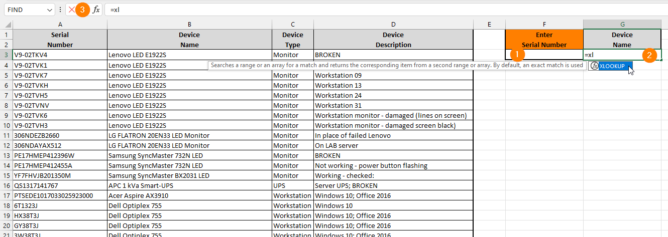
1. We are going to enter the Serial Number we are searching for in cell F2 (leave it blank for now).
2. We are going to enter the XLOOKUP() function in cell G2 and this is where the Device Name is going to be displayed as the result of the function. Type =XL in cell G2 and you will see the XLOOKUP() function appear in the auto-complete list — double-click on the XLOOKUP function
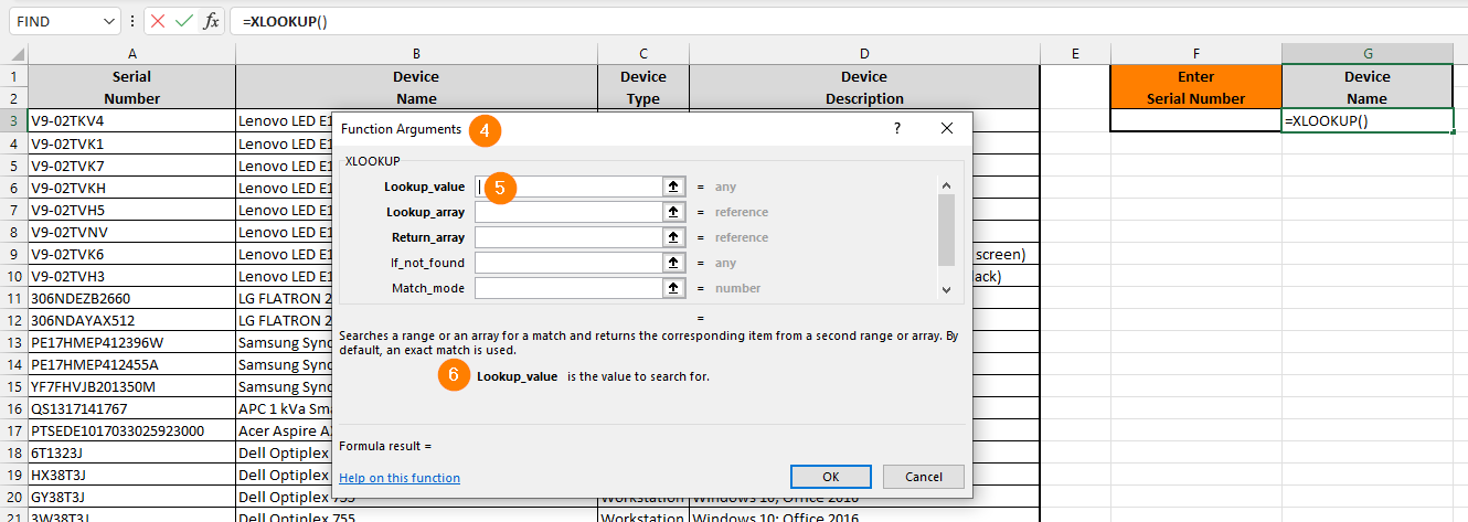
3. Click on the Insert Function button
4. To open the Function Arguments dialog
5. Your cursor should now be in the Lookup_value argument field
6. The description of the Argument that currently has focus

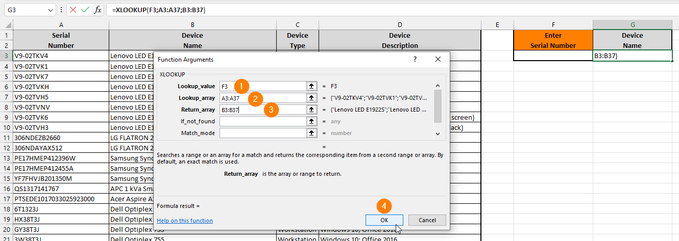
1. The Lookup_value is set to F2 which is where the Serial Number will be entered; this is identical to the first argument of the VLOOKUP() function
2. The Lookup_array is the array which will be searched for the Lookup_value: A3:A37; note that in the VLOOKUP() this second argument is Lookup_table and not Lookup_array
3. The Return_array is the array from which the Device Name will be returned: B3:B37
4. Click the OK button (the remainder of the arguments are optional in this instance)

The final function in G3 is: =XLOOKUP(F3;A3:A37;B3:B37)

2.2 Test

Enter one of the Serial Numbers in cell F3 and confirm that the correct Device Name appears in G3.

Test to see what happens when you modify the functions to read as follows:

=XLOOKUP(F3;A3:A36;B3:B37)

=XLOOKUP(F3;A3:A37;B4:B38)

2.3 Compared to VLOOKUP?

We can — and I recommend you do — achieve the above using VLOOKUP() combined with IFNA().

3. Closest Match

The below example is the equivalent of the VLOOKUP() Closest Match.

1. The Lookup_value is the mark we are searching for
2. The lookup Lookup_array is the range in which to search for the Lookup_value
3. The Return_array is the range from which the Symbol should be returned
4. Match_mode depends on how the Lookup_array is arranged
5. Click the OK button

References:

1. Use the XLOOKUP function – Microsoft Support (2023). Available at: https://support.microsoft.com/en-au/office/xlookup-function-b7fd680e-6d10-43e6-84f9-88eae8bf5929 (Accessed: 16 July 2023).